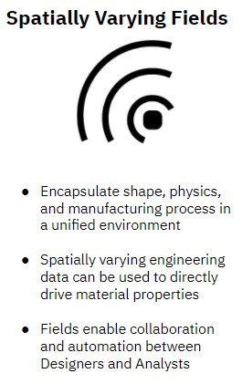
Objective:

Learn how to use ramps and implicit bodies to define a field of engineering data that can be used as inputs into a simulation analysis.

Procedure:

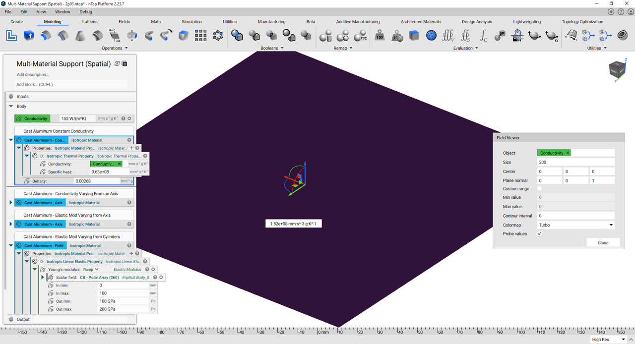
Constant Field:

Traditionally, material properties are defined with constant values. nTop defines scalar engineering values as Scalar Fields. In the figure below, you can see that the Thermal Conductivity is set at 152 W/(m*K) and results in a field that does not change.

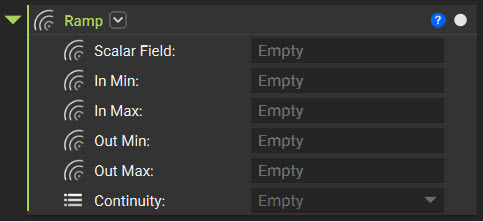
Transforming Distance Fields to Engineering Scalar Fields using the Ramp Block:

By using the Ramp Block, you can use an input field to spatially transform field data into engineering units. This functionality bridges the divide between a field and engineering data and allows complex analysis.

Using this functionality you can the Thermal Conductivity now varies from 152-200 W/(m*K) at a distance from 0-100 mm from the Axis Location.

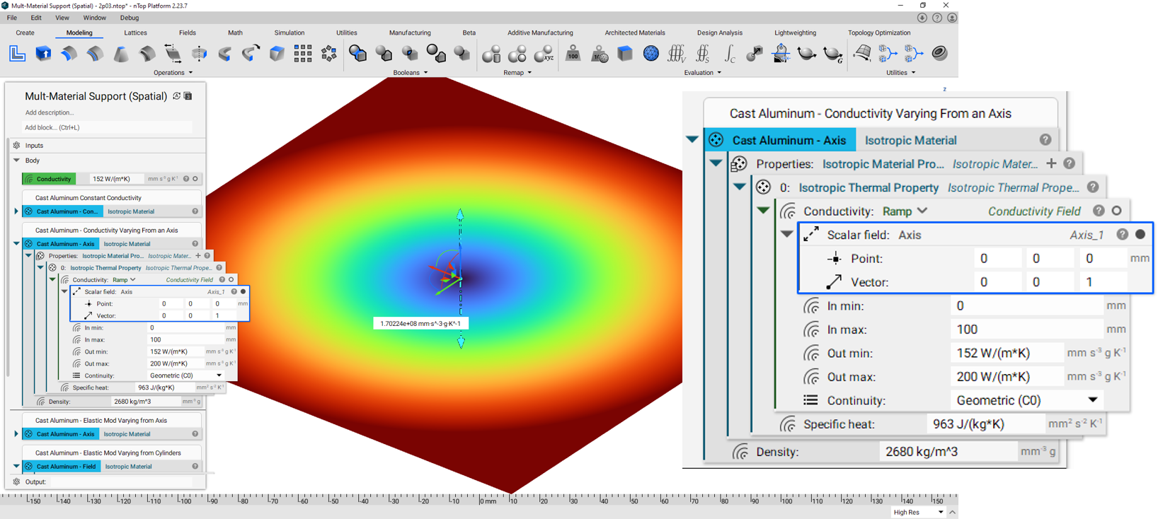
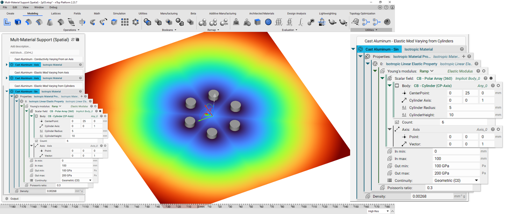
Varying Field using Multiple Objects:

Similarly, you can use multiple implicit bodies with the ramp block to produce more complex field patterns.  In this case, an array of cylinders are used.

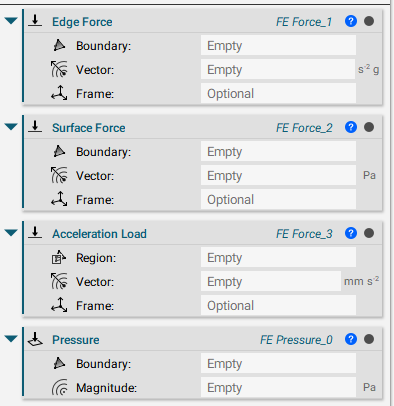
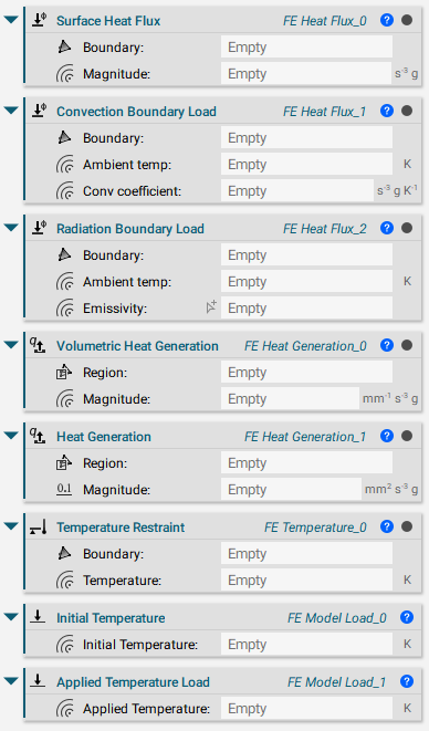
Boundary Conditions:

Just like material properties, certain FEA boundary conditions can vary using scalar field inputs.  Examples of these types are shown below.

Structural Boundary Conditions with Field Inputs	Thermal Boundary Conditions  with Field Inputs

In this instance, convection coefficients can easily be varied using the Ramp block, in the same manner, shown for spatially varying material properties.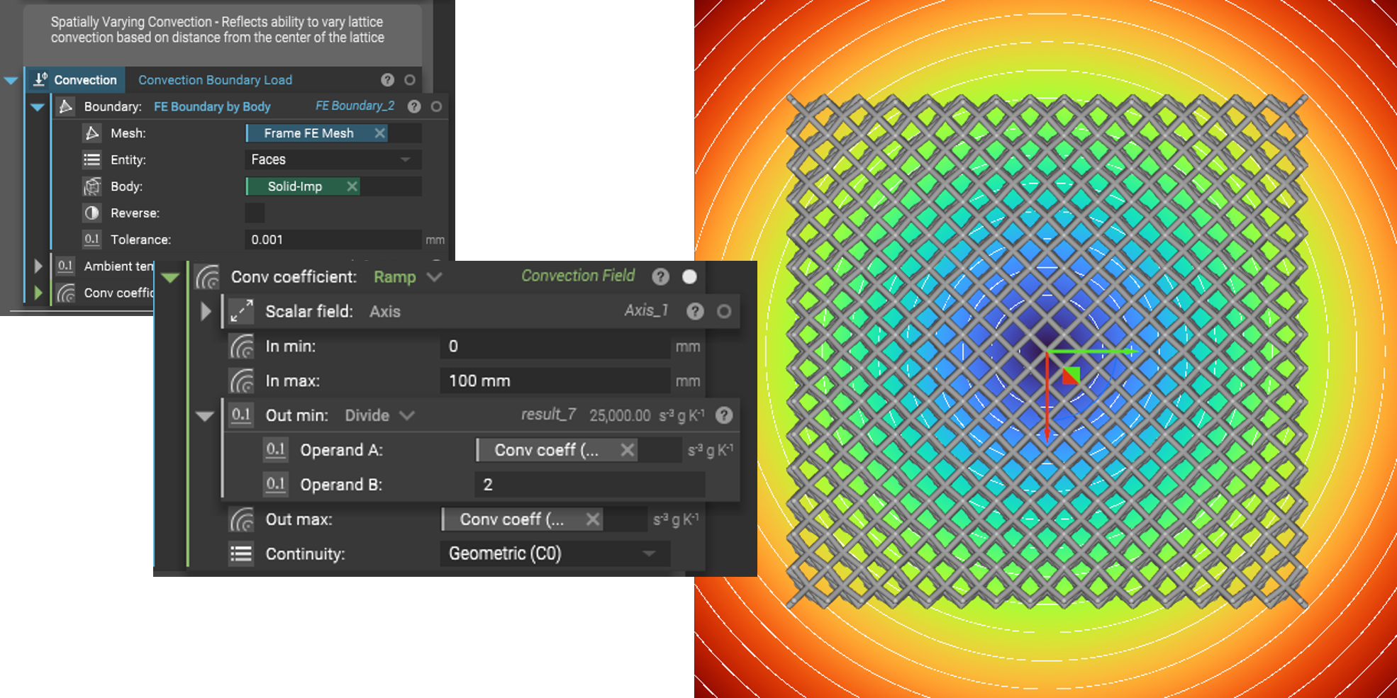  

And that’s it! You’ve successfully defined varying structural and thermal material properties using fields. 

Are you still having issues? Contact the support team, and we’ll be happy to help!

Download the Example file:

• Example file

More on this topic:

• How do I set up a simulation?
• How does the ramp block work?
• How to use simulation results to create a Point Map or Field